Bonds are key to a well-diversified portfolio; they’ve provided both consistent returns and consistent diversification against riskier asset classes like stocks and real estate. But bonds face stiff headwinds in the coming years. That’s not prognostication, it’s a mathematical certainty. It’s imperative that our portfolio designs account for this less optimistic future. Failing to do so ensures that we’ll also fail to meet our goals and expectations.
In this post, we model various future scenarios for the largest class of bond ETFs, US Treasuries, and discuss how investors can succeed in this more challenging future.
But first, a look backwards:
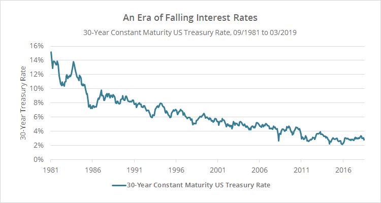
Let’s look at the 30-year US Treasury rate since its peak in 09/1981. Yields have consistently fallen for nearly four decades and now stand near historic lows. We could paint a similar chart for other shorter Treasury durations.
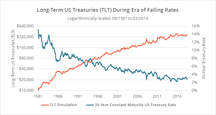
Compare this to the performance of an asset like TLT that closely tracks these rates, over the same period. In the graph below, simulated TLT returns have been painted orange (left axis) and 30-year Treasury rates blue (right axis). Note the consistency with which rates have fallen and TLT would have risen.
For brevity, we’ve skipped the math used to calculate TLT’s simulated performance pre-07/2002, but interested readers can learn more in the notes at the end of this post. The numbers are solid.
TLT would have returned about 10% annually. That’s a near equity-like return, without nearly the same degree of risk and volatility.
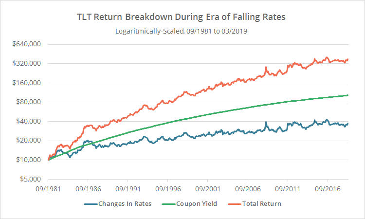
There are two main drivers of returns for Treasury ETFs like TLT: changes in interest rates (declining rates drive prices up, and vice-versa), and the coupon payment itself. The former benefits from falling rates, and the latter benefits from high rates, regardless of whether they’re rising or falling.
How much of the gain in TLT over the last 37+ years was a result of each of those return drivers?
The graph below breaks down TLT’s total return (orange) by whether they were the result of changes in rates (blue) or the coupon yield (green). Note how rate changes are responsible for TLT’s volatility, but the coupon yield provided most of the meat (again, see the end notes to understand the math).
In short, falling interest rates are good. High interest rates (independent of direction) are even better.
Looking forward – a bleak future of rising interest rates:
Unlike periods of rising rates like the 1970’s, an increase in rates today is occurring from a “low base”. Recall from our previous chart that the majority of TLT’s gains have come from high rates. How might Treasury ETFs perform if they’re now rising without a high coupon to offset that change?
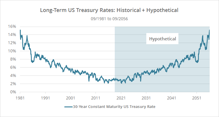
Here’s a thought experiment to answer that question. What if rates marched upwards over the next 37+ years in the reverse order that they fell over the previous 37? In other words, what if rates looked like this:
There’s no reason to expect that to be the case. Rates tend to rise and fall at different speeds and for entirely different reasons. This is simply an attempt to model the interplay between the two main drivers of return in a rising rate environment.
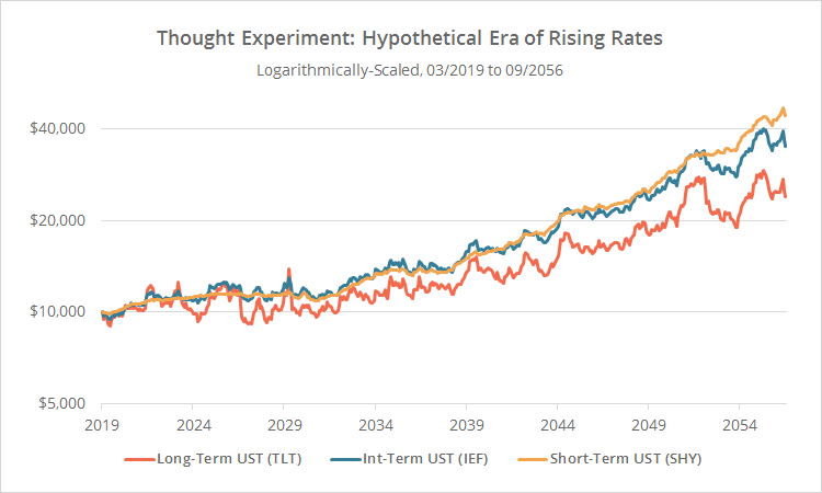
Below we’ve simulated future returns for three US Treasury ETFs: TLT (long-term, 20+ years), IEF (intermediate-term, 7-10 years) and SHY (short-term, 1-3 years).
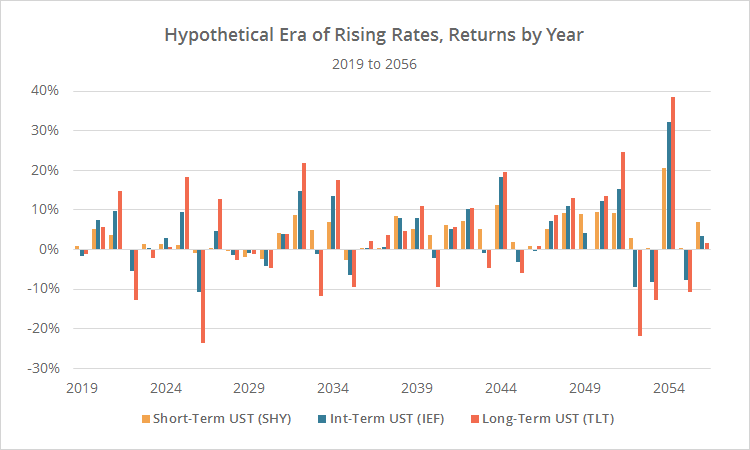
Returns are essentially flat for the next 12 years. Below we show returns by year for our three assets. Note that Treasuries would not become consistently profitable again until about 2031.
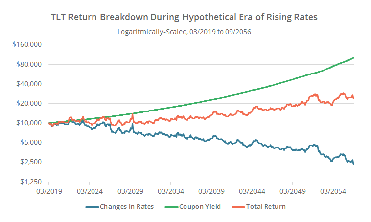
If coupon yield has been the biggest return driver historically, why do these Treasury assets perform so poorly in our hypothetical era of rising interest rates? Because unlike the rising rate environment of the 1970’s, yields are so low today that they can’t make up for rising rates’ drag on bond prices.
To illustrate, below we show the same return breakdown for TLT that we looked at previously. Note how the change in rates (blue) is a constant drag on performance that the initially anemic coupon (green) can’t cover.
Looking forward – a meh future of unchanged interest rates:
What if, instead of rising over the next 37+ years, interest rates simply remained exactly where they were? What sort of annual returns could we expect in the coming years?
The answer is (roughly) the current constant maturity rate. That’s a far lower return than investors are accustomed to. To illustrate, in the table below we show each Treasury ETF’s historical annual return versus current rates. The difference is the annual shortfall investors could expect relative to what they’ve grown accustomed to over the last 37 years.
Rates can’t remain unchanged forever, so this is obviously an unrealistic example, but it illustrates that sideways rates still spell subpar returns for Treasury ETFs.
Practically speaking, rates can’t fall much further from here, but for the curious: What if rates fell to zero in the coming years? How would Treasury ETFs perform in this hypothetical scenario? Pretty good in the very short-term, but terrible in the long-term.
If rates fell to zero (linearly) over the course of the next 5-years, our three ETFs would return about 2.4%, 5.9% and 16.4% per year. That’s great. But then after that no coupon, nada. And any increase in rates would be devastating for returns.
So the future is bleak. What do we do about that?
We know that bonds will underperform what investors have grown accustomed to. Most financial analysis does not adjust for this fact. It naively uses past returns to project future returns. It’s extremely rare in this business that we can say with mathematical certainty that a given asset class will underperform, but this is one of those few instances where we can.
Bonds are still key to a well-diversified portfolio. There are few good options for providing consistent diversification against riskier asset classes like stocks and real estate. But if we over-weight bonds, assuming that they’ll provide the same returns coupled with low risk that they have in the past, we’re setting ourselves up for disappointing results.
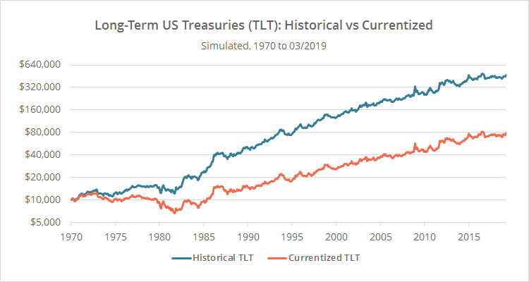
We take a different approach. Our portfolios are designed by “currentizing” historical bond returns. Things get a bit technical from here, but in a nutshell, we deconstruct each bond asset’s history into all of the constituent factors that drive returns. We assume that the largest driver of bond returns, the current yield, was never higher than it stands today. We leave all other return drivers untouched.
Below we show historical returns for long-term US Treasuries (TLT) in blue, versus returns that have been currentized based on where interest rates stand today (03/2019) in orange. The difference is stark, with annual returns cut in half, and a deep drawdown of -47% in the early 1980’s.
This currentizing process means that our asset allocations will slowly change over time based on where yields stand today. That’s okay. Sound buy and hold investing requires periodically rebalancing our portfolio. Those rebalances provide the opportunity to keep up with the optimal allocation. We can also adjust to the optimal allocation when we add funds (by buying assets that we’re under-allocated to) or withdraw funds (by selling assets that we’re over-allocated to).
There are no magic answers to a future of mediocre bond performance. Bonds will always be key to building a diversified portfolio, but it’s imperative that our portfolio designs account for this less optimistic future. Failing to do so ensures that we’ll also fail to meet our goals and expectations.
We invite you to learn more about our process and take our Portfolio Builder for a free test drive. Become a member for less than a $1 a week to unlock all functionality. Have questions? Please check out our FAQs or contact us.
Calculation notes:
We simulated returns for constant maturity instruments using the formula below. This example uses monthly interval data. For simplicity, we’ve ignored fund expenses and other less significant return drivers.
currentPrice = previousPrice * (((((previousRate * (1 – (1 + currentRate) ^ (maturityYears * -1)) / currentRate) + (1 / (1 + currentRate) ^ maturityYears) – 1)) + (average(previousRate, currentRate) / 12)) + 1)
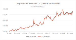 The first half of the formula estimates the price change from changes in rates; the latter half the price change from the coupon yield.
In the graph to the right (click to zoom), we show the actual TLT (grey) versus our simulation (orange) since TLT’s inception. Note the tight fit (correlation = 99.3%). We see a similar high degree of fit comparing our simulation to other relevant indices with longer histories like DBUS20VL.
- This modelling approach is only accurate for instruments adhering to approximately the “constant maturity” yield, which practically speaking, nearly all US Treasury ETF/mutual funds do.
- Modelling returns based on yields for non-Treasury assets like corporate bonds is more difficult and much less precise, but the fundamental conclusion of this post still holds.
